Download or preview the pdf file below with instructions for the Portfolio tasks.
CC1: Hosting - Display charts in your own site
The following charts were built with data from Richard Davies's GitHub repository
and inspired by the charts in his library.
Hoover over them for additional information about data points.
I chose topics related to social issues, such as the Glasgow Effect (life expectancy and deprivation) and school enrollment gaps by gender.
Figure 1Figure 2
CC2: Building - Create your own visualisations
From the Economics Observatory Data Hub,
I chose two other charts to reproduce them within my own adapted json codes.
Click on the upper right corner of each chart to go to each json file, visualized in VegaLite.
Figure 3Figure 4
CC3: Debating - Use a visualisation in economic/policy commentary
From the Festival of Economics 2024
I created two charts focusing on the Marshall Paley Lecture about inequalities, where Professor Sir Richard Blundell
discussed different dimensions and dynamics in that field.
Figure 5
From the second chart, growth incidence curves in the UK show highly regressive dynamics in 1982-1992 and more progressive
ones from then on. Nevertheless, there was a setback from 2002-2012 to 2012-2022, where lower percentiles did not enjoy
as much growth relatively compared to the previous decade.
Figure 6
CC4: Replication - Re-create, then improve, someone else’s chart
From the
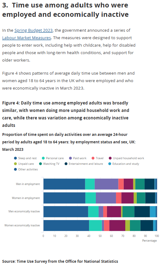
ONS's site about time use in the UK, I selected the following chart (Figure 7).
Figure 7
Then, I replicated their chart and changed several features that seemed better for me to be displayed in other ways.
For instance, I avoided stacking bars and, instead, I chose to divide by activities for a better understanding of the relative differences by gender.
Figure 8
CC5: Scraper - Implement a data scraper of your own
I chose the Child Penalty Atlas website as it has valuable analysis of the gender dynamics behind labour penalization for becoming parents.
This is not a negative view of parenthood but a call for attention for labour markets and intrahousehold allocations to rebalance their outcomes.
I developed this topic further in my Project.
I scrapped data from their website and cleaned it on a GoogleColab file.
Figure 9
CC6: Loops - Build a dashboard
I used the ONS API to batch download nine series as json files using a loop. In this
GoogleColab file
I conducted the data analysis to create the following charts.
Figure 10
CC7: Maps - Base maps and choropleths
I produced two maps of Chile, one showing the different regions with their municipalities' borders and the other plotting population by each municipality. From both maps, we can see how different regions consider very different lands in terms of geographical scope and latitude. Then we see, in Figure 12, that some municipalities, such as Antofagasta, are very populated while covering a large geographical space. In contrast, others from the capital of Chile (Santiago), such as La Florida, have similar populations but in a much smaller area.
Figure 11Figure 12
CC8: Analytics charts
The following charts use coloured scatter techniques for three-dimensional analysis. I chose the topic of parenthood leaves
to assess the relationship between mothers' and fathers' available days, along with an additional feature, either Gender Wage Gap, Share of women in
high management positions, or universal health coverage levels. The main finding here is that health coverage plays a more significant role when relating to
leaves than measures of women's power. Codes that manage data can be found in here.
Figure 13Figure 14Figure 12
CC9: Big Data - Extracting a story from millions of prices
I used price data from Richard Davies's GitHub, transformed it in Google Colab to identify pairs of items that share descriptions but
were specified for women or men. I averaged shop prices by region, and then used the output dataset to generate a JSON chart grid.
The prices are smoothed using a moving average and restricted until 2006 for comparison. The motivation was common literature on
gendered prices or the better-known
"Pink tax", although I found no evidence of that for the selected item (leather boots).
Figure 13
CC10: Machine Learning
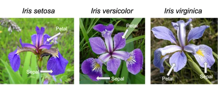
The image in Figure 14 comes from a selected website, and shows three species of flowers that look similar but differ on the lenght and width of their petals and sepals.
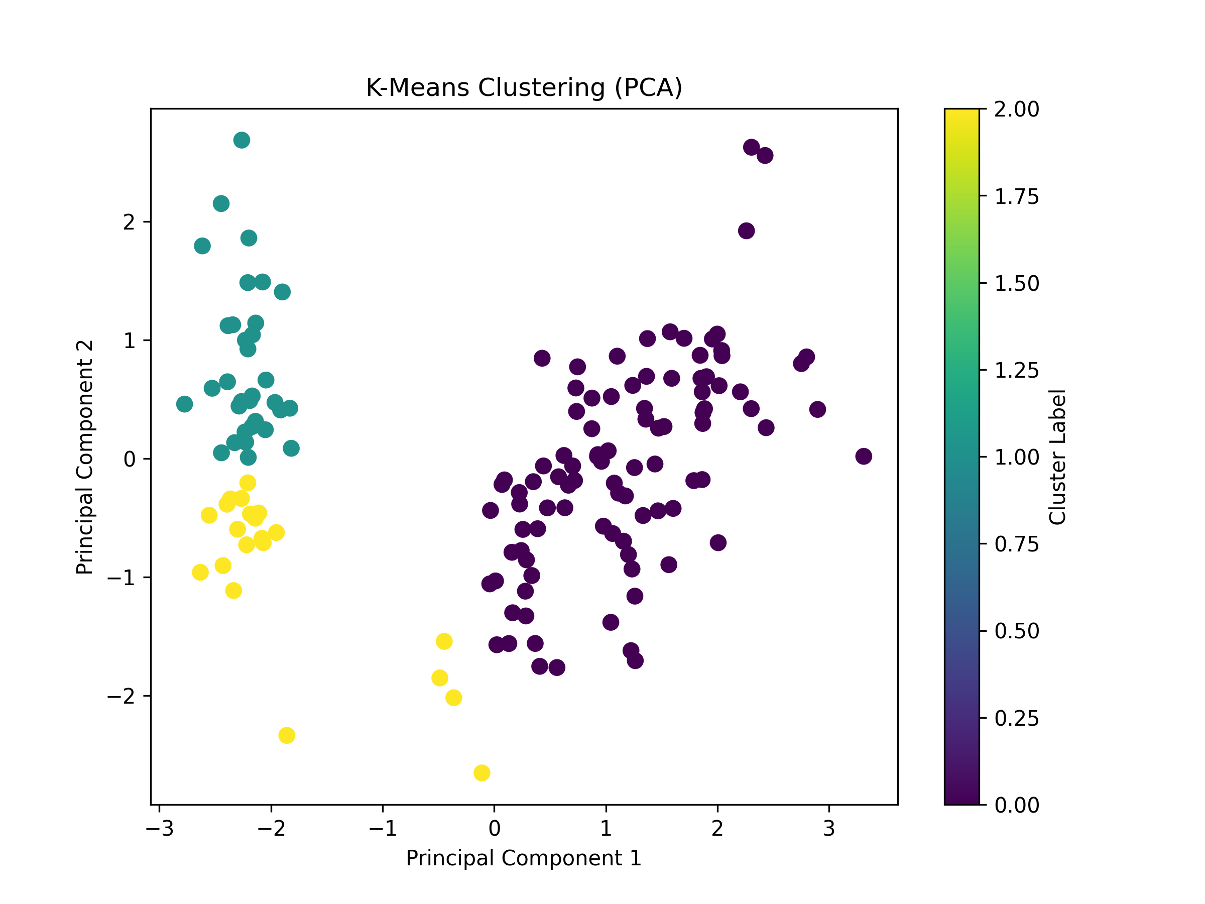
First I performed an unsupervised learning method. I used a Google Colab code to load the data,
standarize it, and apply a K-Means Clustering (with three clusters, knowing that we want to identify three species of flowers). I then plot the PCA results in Figure 15, along with comparing resulting clusters
with true labels, and observe that one species (cluster 1) was identified correctly (with 33 samples of label 0 setosa), but the two (versicolor and virginica) others were not, so K-Means (PCA) has some limitations for this analysis.
Figure 14
Figure 15
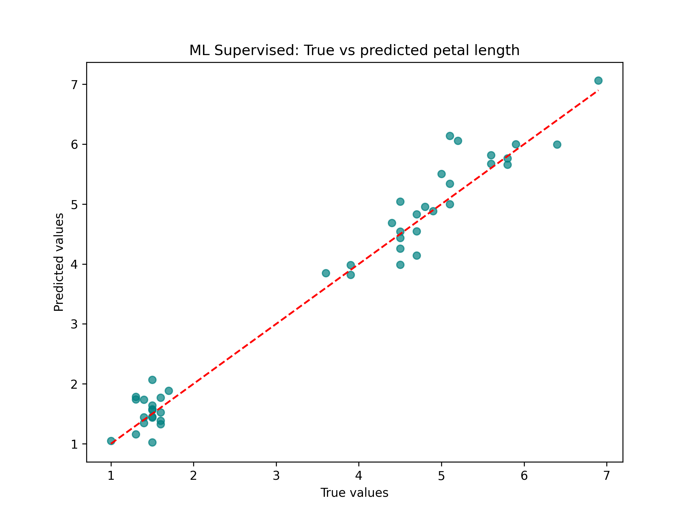
Then I performed a supervised ML based on a linear regression analysis, shown in Figure 16. The corresponding code is on Google Colab